MOLONARI-1D
Introduction
This page is a first dive into the MOLONARI-1D device for people who want to understand the science behind it and deploy their own sensor.
The MOLONARI project can be separated into two main parts, that will be detailed as you read:
Computing
Understanding the equations behind MOLONARI
1. Aquifers
Have you ever dug a hole on the beach to imprison your siblings or your parents? If so, you know that after digging for a while, the sand becomes darker, heavier and wetter: this is because water has infiltrated the sand.
Surprisingly, this is the case everywhere on Earth. Water infiltrates the soil and geological layers under our feet, from top to bottom, until it finds an impermeable layer. The geological layers that host water are made of small grains like clay (~0.5 μm) and sand (~0.5 mm). They are called the matrix, and the matrix filled with water is called an aquifer.
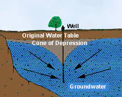
This water, although slowed by the matrix, can flow. Because of gravity, the water level tends to flatten itself: this is why digging a deep hole (10-30 m) is enough to build a well!
Because water flows in the aquifer, the aquifer exchanges water with its nearby mediums: rivers, oceans, and rainfall. Thus, the water level varies. A low water level corresponds to a period of drought, and a high water level can be observed after a period of rains and water infiltration.
2. The hydraulic head
This is what the Molonari project tries to monitor: how do rivers and aquifer interact? How much water is exchanged, and in what direction?
This question is not new; and since the 19th century, scientists and engineers have laid out the foundations of a science of the underground water: hydrogeology.
At the heart of this science is an important measurement, called the hydraulic head. Expressed in meters, this measurement combines the water’s height, pressure and kinetic energy in order to ease the understanding of water flows: the higher the head, the more the water wants to “go down”. The water of an aquifer with a high head will eventually “push” the water of a neighbor aquifer with a low head, until the heads balance together. In an aquifer, water has almost no kinetic energy, so the hydraulic head is defined as
\(h = z+\frac p {\rho g} \)
where \(z\) is the height of the particle of water, \(p\) the pressure around, \(\rho\) the volumic mass of water and \(g\) the gravity acceleration constant.
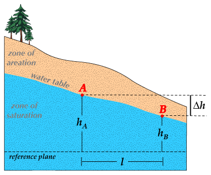
In this example, \(h_A > h_B\) so the water flows from A to B.
Source: https://punchlistzero.com/hydraulic-gradient/
3. Darcy speed
Now, how do we express the fact that water flows in an aquifer? We already assumed that a water particle had no kinetic energy: thus, we use the flow.
The Darcy law links the surficial water flow \(\overrightarrow q\) (\(m.s^{-1}\)) with the hydraulic head, where \(K\) (\(m.s^{-1}\)) is the hydraulic conductivity of the medium.
\(\overrightarrow q=-K\overrightarrow\nabla h\)
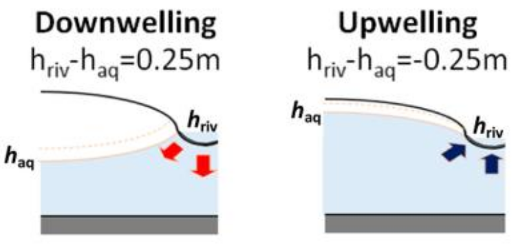
For example, if water flows from the river to the aquifer, the surficial water flow should be oriented towards negative altitudes (\(-e_z\)). Otherwise, if water flows from the aquifer to the river, the surficial water flow should oriented towards positive altitudes, meaning that the hydraulic charge is lower in the river than in the aquifer.
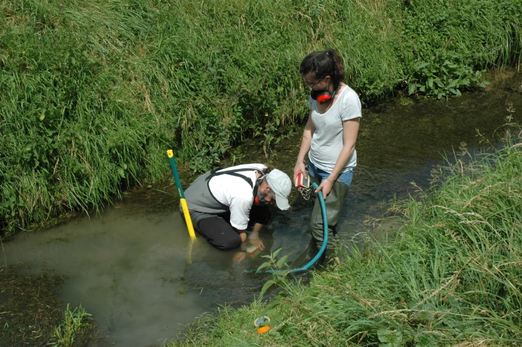
Assuming that we know \(K\), we simply have to measure the hydraulic head at two different altitudes of the same water column under the river to know the flow! This is done using a differential pressure sensor, that compares the pressures at the bottom of the river and 40cm below the riverbed. We can then compute \(\overrightarrow\nabla h\) between these two points and derive \(\overrightarrow q\).
4. Determining \(K\)
The problem is that \(K\) varies between mediums… a lot: in gravel, K ~ 30 cm/s, wheras is clay, K ~ 50 nm/s. We need another equation to compute this hydraulic conductivity.
For that, we have to consider heat exchanges under the riverbed. The heat equation can be written as follows:
\(\frac{\partial\theta}{\partial t}=\kappa_e \Delta\theta+\alpha_e \nabla h \nabla \theta\)
where \(\kappa_e=\frac{\lambda_m}{\rho_mc_m}\) and \(\alpha_e=\frac{\rho_wc_w}{\rho_mc_m}K\) are parameters that depend on the thermal conductivity \(\lambda\), thermal capacity \(c\), intrinsic permeability \(k\), volumic mass \(\rho\) and porosity \(n\) of the medium and water. Some of them we know, some of them we don’t.
We can interpret the heat equation as a sum of two heat flows: the conductive flow \(-\lambda\nabla\theta\), which happens naturally with matter, and the advective flow \(q \rho_wc_w\theta\) which happens only when the liquid is moving.
Now, how can we use this new equation to derive \(K\)?
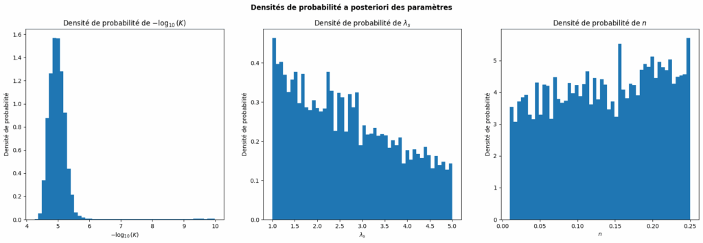
5. Markov Chains and Bayesian Inversion
First, we want to measure \(\theta\) and its evolutions at different points of the water column. For that, the MOLONARI team chose to add four temperature sensors at variable depths: every 10 centimeters.
We then compile this temperature and pressure data with a Bayesian inversion in order to know the parameters of the medium. The idea of the algorithm, called a Markov chain, is as follows:
- First, we choose a set of parameter values for the medium \((K, \lambda_m, n)\) that are acceptable, i.e. within the value range that we know they belong to.
- For each one of these parameters sets, we solve the heat equation to get the theoretical temperature profile that we would get with these parameters.
- We compare each temperature profile with the actual temperature data.
- When the error is big, we eliminate this parameter set, for we know that it yields inaccurate temperatures.
- When the error is small, we keep this parameter set and we generate parameters sets by adding randomized deltas to each one of these parameters.
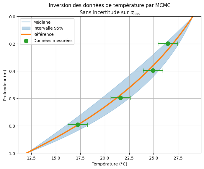
By iterating this process on and on, the parameters distribution should converge. The resulting distributions are called a posteriori distributions, and their maxima correspond, with a certain probability, to the value of the parameter of the medium. In other words, we now know the most probable values for \(K\), \(\lambda_m\), and \(n\).
The following graph shows how well the Markov chain converges to temperature profiles that are close to the reference temperature profile (in orange). The process only knows the green values and outputs the blue curve.
Hardware
Building the sensors
1. Overall Architecture
Now that we understand the equations, we need to build a device that provides:
- A differential pressure sensor between the riverbed and the aquifer (~40cm in depth)
- 4 temperature sensors at variables depths under the riverbed (~10, 20, 30, 40cm in depth)
The current MOLONARI-1D device fulfills these conditions with two different modules: one for the differential pressure, the other one for the temperatures. In 2025, we have been working on a single device that could embed both.
The devices are each run by an Arduino board that sends data to a nearby receiver, through an Internet of Things (IoT) Wi-Fi protocol. This receiver then sends the data again to a remote server through the Internet. This in-between receiver allows us to gather the data in real-time, and to know whenever there is a problem on one of the probes.
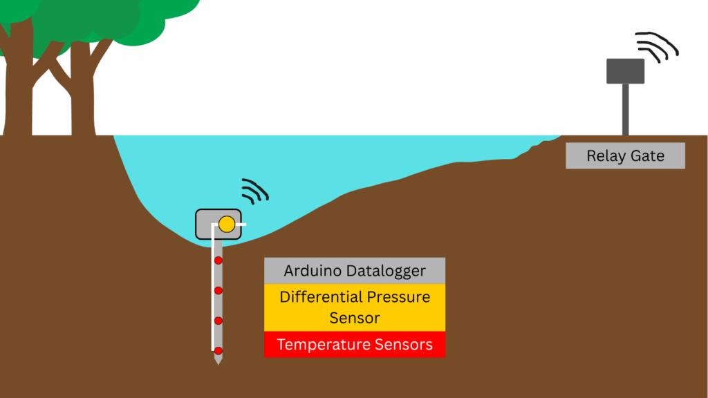
In the 2025 design, temperature and pressure sensors belong to a single probe.